Problem Set 4 (SOLUTIONS)
This problem set will revisit some of the material covered in Handouts 3 and 4. You will be required to work with a ‘raw’ dataset, downloaded from an online repository. For this reason, you should take care to check how the data is coded.
You will be using a version of the US Current Population Survey (CPS) called the Merged Outgoing Rotation Group (MORG). This data is compiled by the National Bureau of Economic Research (NBER) and has been used in many famous studies of the US economy. The CPS has a rather unique rotating panel design: “The monthly CPS is a rotating panel design; households are interviewed for four consecutive months, are not in the sample for the next eight months, and then are interviewed for four more consecutive months.” (source: IPUMS). The NBER’s MORG keeps only the outgoing rotation group’s observations.
The MORG .dta files can be found at: https://data.nber.org/morg/annual/.
Preamble
Create a do-file for this problem set and include a preamble that sets the directory and opens the data directly from the NBER website. Of course, this requires a good internet connection. For example,
clear
//or, to remove all stored values (including macros, matrices, scalars, etc.)
*clear all

* Replace $rootdir with the relevant path to on your local harddrive.
cd "$rootdir/problem-sets/ps-4"

cap log close
log using problem-set-4-log.txt, replace

use "https://data.nber.org/morg/annual/morg19.dta", clear
You can, of course, download the data and open it locally on your computer.
Questions
1. Create a new variable exper equal to age minus (years of education + 6). This is referred to as potential years of experience. Check how each variable defines missing values before proceeding. You will need to create a years of education variable for this. Here is he the suggested code:
tab grade92, m
gen eduyrs = .
    replace eduyrs = .3 if grade92==31
    replace eduyrs = 3.2 if grade92==32
    replace eduyrs = 7.2 if grade92==33
    replace eduyrs = 7.2 if grade92==34
    replace eduyrs = 9  if grade92==35
    replace eduyrs = 10 if grade92==36
    replace eduyrs = 11 if grade92==37
    replace eduyrs = 12 if grade92==38
    replace eduyrs = 12 if grade92==39
    replace eduyrs = 13 if grade92==40
    replace eduyrs = 14 if grade92==41
    replace eduyrs = 14 if grade92==42
    replace eduyrs = 16 if grade92==43
    replace eduyrs = 18 if grade92==44
    replace eduyrs = 18 if grade92==45
    replace eduyrs = 18 if grade92==46
    lab var eduyrs "completed education"
tab grade92, sum(eduyrs)
    Highest |
      grade |
  completed |      Freq.     Percent        Cum.
------------+-----------------------------------
         31 |        814        0.28        0.28
         32 |      1,495        0.51        0.79
         33 |      3,071        1.05        1.85
         34 |      4,123        1.41        3.26
         35 |      5,244        1.80        5.06
         36 |      7,824        2.69        7.75
         37 |      9,271        3.18       10.93
         38 |      4,226        1.45       12.38
         39 |     82,795       28.41       40.79
         40 |     50,112       17.20       57.99
         41 |     12,392        4.25       62.24
         42 |     16,161        5.55       67.79
         43 |     59,438       20.40       88.19
         44 |     25,374        8.71       96.89
         45 |      3,785        1.30       98.19
         46 |      5,265        1.81      100.00
------------+-----------------------------------
      Total |    291,390      100.00
(291,390 missing values generated)
(814 real changes made)
(1,495 real changes made)
(3,071 real changes made)
(4,123 real changes made)
(5,244 real changes made)
(7,824 real changes made)
(9,271 real changes made)
(4,226 real changes made)
(82,795 real changes made)
(50,112 real changes made)
(12,392 real changes made)
(16,161 real changes made)
(59,438 real changes made)
(25,374 real changes made)
(3,785 real changes made)
(5,265 real changes made)

    Highest |
      grade |   Summary of completed education
  completed |        Mean   Std. dev.       Freq.
------------+------------------------------------
         31 |   .30000001           0         814
         32 |         3.2           0       1,495
         33 |   7.1999998           0       3,071
         34 |   7.1999998           0       4,123
         35 |           9           0       5,244
         36 |          10           0       7,824
         37 |          11           0       9,271
         38 |          12           0       4,226
         39 |          12           0      82,795
         40 |          13           0      50,112
         41 |          14           0      12,392
         42 |          14           0      16,161
         43 |          16           0      59,438
         44 |          18           0      25,374
         45 |          18           0       3,785
         46 |          18           0       5,265
------------+------------------------------------
      Total |   13.556855   2.7030576     291,390
tab age, m
gen exper = age-(eduyrs+6)
        Age |      Freq.     Percent        Cum.
------------+-----------------------------------
         16 |      4,661        1.60        1.60
         17 |      4,630        1.59        3.19
         18 |      4,417        1.52        4.70
         19 |      4,039        1.39        6.09
         20 |      3,915        1.34        7.43
         21 |      3,996        1.37        8.81
         22 |      3,918        1.34       10.15
         23 |      3,950        1.36       11.51
         24 |      4,194        1.44       12.94
         25 |      4,185        1.44       14.38
         26 |      4,325        1.48       15.87
         27 |      4,476        1.54       17.40
         28 |      4,600        1.58       18.98
         29 |      4,633        1.59       20.57
         30 |      4,829        1.66       22.23
         31 |      4,735        1.62       23.85
         32 |      4,601        1.58       25.43
         33 |      4,748        1.63       27.06
         34 |      4,646        1.59       28.66
         35 |      4,730        1.62       30.28
         36 |      4,742        1.63       31.91
         37 |      4,848        1.66       33.57
         38 |      4,550        1.56       35.13
         39 |      4,735        1.62       36.76
         40 |      4,667        1.60       38.36
         41 |      4,503        1.55       39.90
         42 |      4,390        1.51       41.41
         43 |      4,309        1.48       42.89
         44 |      4,193        1.44       44.33
         45 |      4,253        1.46       45.79
         46 |      4,266        1.46       47.25
         47 |      4,447        1.53       48.78
         48 |      4,563        1.57       50.34
         49 |      4,698        1.61       51.96
         50 |      4,646        1.59       53.55
         51 |      4,477        1.54       55.09
         52 |      4,555        1.56       56.65
         53 |      4,523        1.55       58.20
         54 |      4,736        1.63       59.83
         55 |      5,010        1.72       61.55
         56 |      5,035        1.73       63.27
         57 |      4,976        1.71       64.98
         58 |      5,030        1.73       66.71
         59 |      5,066        1.74       68.45
         60 |      5,124        1.76       70.20
         61 |      5,067        1.74       71.94
         62 |      5,035        1.73       73.67
         63 |      4,927        1.69       75.36
         64 |      4,892        1.68       77.04
         65 |      4,554        1.56       78.60
         66 |      4,526        1.55       80.16
         67 |      4,344        1.49       81.65
         68 |      4,328        1.49       83.13
         69 |      4,100        1.41       84.54
         70 |      4,058        1.39       85.93
         71 |      4,008        1.38       87.31
         72 |      3,897        1.34       88.65
         73 |      3,147        1.08       89.73
         74 |      2,815        0.97       90.69
         75 |      2,809        0.96       91.66
         76 |      2,623        0.90       92.56
         77 |      2,373        0.81       93.37
         78 |      2,201        0.76       94.13
         79 |      1,977        0.68       94.80
         80 |      7,799        2.68       97.48
         85 |      7,340        2.52      100.00
------------+-----------------------------------
      Total |    291,390      100.00
2. Keep only those between the ages of 18 and 54. Check the distribution of `exper’ and replace any negative values to 0.
keep if inrange(age,18,54)
sum exper, det
replace exper=0 if exper<0
(126,352 observations deleted)
exper
-------------------------------------------------------------
Percentiles Smallest
1% 0 -6
5% 1 -5
10% 2 -4 Obs 165,038
25% 7 -4 Sum of wgt. 165,038
50% 16 Mean 16.50623
Largest Std. dev. 10.57401
75% 25 47.7
90% 31 47.7 Variance 111.8097
95% 34 47.7 Skewness .1296908
99% 36 47.7 Kurtosis 1.887811
(1,078 real changes made)3. Create a categorical variable that takes on 4 values: 1 “less than High School”; 2 “High School Diploma”; 3 “some Higher Education”; 4 “Bachelors”; 5 “Postgraduate”. This variable should be based on the the grade92 variable. You can find the value labels for this variable in this document: https://data.nber.org/morg/docs/cpsx.pdf. I suggest using the recode command, which allows you to create value labels while assigning values. Check the distributio of exper by education category.
recode grade92 (31/38 = 1 "<HS") (39 = 2 "HS") (40/42 = 3 "HS+") (43 = 4 "BA") (44/46 = 5 "PG"), gen(educat)
tab grade92 educat, m

tab educat, sum(exper)
(165,038 differences between grade92 and educat)
Highest |
grade | RECODE of grade92 (Highest grade completed)
completed | <HS HS HS+ BA PG | Total
-----------+-------------------------------------------------------+----------
31 | 398 0 0 0 0 | 398
32 | 578 0 0 0 0 | 578
33 | 1,515 0 0 0 0 | 1,515
34 | 1,571 0 0 0 0 | 1,571
35 | 1,971 0 0 0 0 | 1,971
36 | 2,198 0 0 0 0 | 2,198
37 | 4,373 0 0 0 0 | 4,373
38 | 2,440 0 0 0 0 | 2,440
39 | 0 45,013 0 0 0 | 45,013
40 | 0 0 30,934 0 0 | 30,934
41 | 0 0 7,154 0 0 | 7,154
42 | 0 0 9,708 0 0 | 9,708
43 | 0 0 0 37,557 0 | 37,557
44 | 0 0 0 0 14,804 | 14,804
45 | 0 0 0 0 2,021 | 2,021
46 | 0 0 0 0 2,803 | 2,803
-----------+-------------------------------------------------------+----------
Total | 15,044 45,013 47,796 37,557 19,628 | 165,038
RECODE of |
grade92 |
(Highest |
grade | Summary of exper
completed) | Mean Std. dev. Freq.
------------+------------------------------------
<HS | 19.29665 12.82301 15,044
HS | 17.726435 11.044222 45,013
HS+ | 15.643589 10.806949 47,796
BA | 15.376841 9.3440749 37,557
PG | 15.900092 8.1569821 19,628
------------+------------------------------------
Total | 16.514468 10.560511 165,0384. Create the variable lnwage equal to the (natural) log of weekly earnings. Create a figure that shows the predicted linear fit of lwage against exper, by educat. Try to place all 5 fitted lines in the same graph.
gen lnwage = ln(earnwke)
twoway (lfit lnwage exper if educat==1) (lfit lnwage exper if educat==2)  (lfit lnwage exper if educat==3) (lfit lnwage exper if educat==4) (lfit lnwage exper if educat==5) , legend(order(1 "<HS" 2 "HS" 3 "HS+" 4 "BA" 5 "PG") pos(6) r(1)) xtitle(Years of experience)
(49,686 missing values generated)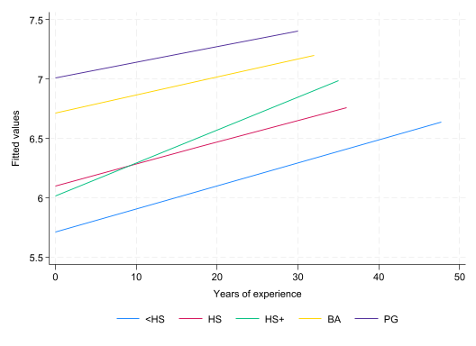
5. Estimate a linear regression model that allows the slope coefficient on exper and constant term to vary by education category (educat). Let the base (excluded) education category be 2 “High School diploma”.
\[ \ln(Wage_i) = \alpha + \sum_{j\neq2}\psi_j \mathbf{1}\{Educat_i=j\} + \beta Exper_i + \sum_{j\neq2}\gamma_j Exper_i\times\mathbf{1}\{Educat_i=j\}+\upsilon_i \]
reg lnwage ib2.educat##c.exper
      Source |       SS           df       MS      Number of obs   =   115,352
-------------+----------------------------------   F(9, 115342)    =   4039.95
       Model |  17435.5509         9  1937.28343   Prob > F        =    0.0000
    Residual |  55310.0589   115,342  .479530951   R-squared       =    0.2397
-------------+----------------------------------   Adj R-squared   =    0.2396
       Total |  72745.6098   115,351   .63064568   Root MSE        =    .69248

------------------------------------------------------------------------------
      lnwage | Coefficient  Std. err.      t    P>|t|     [95% conf. interval]
-------------+----------------------------------------------------------------
      educat |
        <HS  |  -.3882762   .0178644   -21.73   0.000    -.4232902   -.3532622
        HS+  |  -.0839435   .0104229    -8.05   0.000    -.1043722   -.0635149
         BA  |   .6145964   .0109763    55.99   0.000     .5930831    .6361097
         PG  |   .9055692   .0141961    63.79   0.000      .877745    .9333933
             |
       exper |   .0182621   .0003709    49.24   0.000     .0175351    .0189891
             |
      educat#|
     c.exper |
        <HS  |    .001037   .0007627     1.36   0.174     -.000458    .0025319
        HS+  |   .0095156   .0005186    18.35   0.000     .0084991    .0105321
         BA  |  -.0032067   .0005743    -5.58   0.000    -.0043324   -.0020811
         PG  |  -.0051215   .0007698    -6.65   0.000    -.0066302   -.0036128
             |
       _cons |   6.101809   .0077485   787.48   0.000     6.086622    6.116996
------------------------------------------------------------------------------
6. Show that after 13 years of experience, those with some Higer Education (but no Bachelors), out earn those with just a high school diploma. You can assume that there are is a 2 year difference between the experience (education).
dis _b[exper]*14
dis (_b[exper] + _b[3.educat#exper])*12 + _b[3.educat]


dis _b[exper]*15
dis (_b[exper] + _b[3.educat#exper])*13 + _b[3.educat]
.25566943
.24938901
.27393153
.277166727. Use the post-estimation test command to test the null hypothesis: \(H_0: 15\beta = 13(\beta+\gamma_3)+\psi_3\).
test exper*15 = (exper+3.educat#exper)*13+3.educat
 ( 1)  - 3.educat + 2*exper - 13*3.educat#c.exper = 0

       F(  1,115342) =    0.32
            Prob > F =    0.5734
8. Estimate a transformed version of the above model allowing you to test the above hypothesis using the coefficient from a single regressor. That is, the resulting test should be a simple t-test of \(H_0: \phi=0\), where \(\phi\) is the coefficient on the interaction of exper and a dummy variable for educat=3. This will be easier to do if you estimate the model using only the relevant sample: those with High School diplomas and some Higher Education. I suggest avoiding the use of factor notation to create the dummy variables and interaction terms for this exercise. For example, the following should replicate the relevant coefficients from Q5.
gen hasHE = educat==3 if inlist(educat,2,3)
gen hasHEexp = hasHE*exper

reg lnwage exper hasHE hasHEexp
(72,229 missing values generated)
(72,229 missing values generated)
Source | SS df MS Number of obs = 62,811
-------------+---------------------------------- F(3, 62807) = 2860.46
Model | 4000.16053 3 1333.38684 Prob > F = 0.0000
Residual | 29277.0845 62,807 .466143655 R-squared = 0.1202
-------------+---------------------------------- Adj R-squared = 0.1202
Total | 33277.2451 62,810 .529808073 Root MSE = .68275
------------------------------------------------------------------------------
lnwage | Coefficient Std. err. t P>|t| [95% conf. interval]
-------------+----------------------------------------------------------------
exper | .0182621 .0003657 49.94 0.000 .0175453 .0189789
hasHE | -.0839435 .0102764 -8.17 0.000 -.1040852 -.0638019
hasHEexp | .0095156 .0005113 18.61 0.000 .0085134 .0105178
_cons | 6.101809 .0076396 798.71 0.000 6.086835 6.116782
------------------------------------------------------------------------------gen experR = exper+hasHEexp*2/13
gen hasHER = hasHE-hasHEexp/13
reg lnwage experR hasHER hasHEexp(72,229 missing values generated)
(72,229 missing values generated)
Source | SS df MS Number of obs = 62,811
-------------+---------------------------------- F(3, 62807) = 2860.46
Model | 4000.16052 3 1333.38684 Prob > F = 0.0000
Residual | 29277.0845 62,807 .466143655 R-squared = 0.1202
-------------+---------------------------------- Adj R-squared = 0.1202
Total | 33277.2451 62,810 .529808073 Root MSE = .68275
------------------------------------------------------------------------------
lnwage | Coefficient Std. err. t P>|t| [95% conf. interval]
-------------+----------------------------------------------------------------
experR | .0182621 .0003657 49.94 0.000 .0175453 .0189789
hasHER | -.0839435 .0102764 -8.17 0.000 -.1040852 -.0638019
hasHEexp | .0002489 .0004358 0.57 0.568 -.0006053 .001103
_cons | 6.101809 .0076396 798.71 0.000 6.086835 6.116782
------------------------------------------------------------------------------9. Verify that the F-statistic from Q7 is the square of the above T-statistic.
dis (_b[hasHEexp]/_se[hasHEexp])^2.3261014310. Use the restricted OLS approach to replicate the F-statistic and p-value from Q7.
reg lnwage exper hasHE hasHEexp
scalar RSSu = e(rss)
scalar DOFu = e(df_r)
reg lnwage experR hasHER
scalar RSSr = e(rss)
scalar DOFr = e(df_r)

scalar Fstat = ((RSSr-RSSu)/(DOFr-DOFu))/(RSSu/DOFu)
scalar pval = Ftail(1,DOFu,Fstat)

scalar list Fstat pval
      Source |       SS           df       MS      Number of obs   =    62,811
-------------+----------------------------------   F(3, 62807)     =   2860.46
       Model |  4000.16053         3  1333.38684   Prob > F        =    0.0000
    Residual |  29277.0845    62,807  .466143655   R-squared       =    0.1202
-------------+----------------------------------   Adj R-squared   =    0.1202
       Total |  33277.2451    62,810  .529808073   Root MSE        =    .68275

------------------------------------------------------------------------------
      lnwage | Coefficient  Std. err.      t    P>|t|     [95% conf. interval]
-------------+----------------------------------------------------------------
       exper |   .0182621   .0003657    49.94   0.000     .0175453    .0189789
       hasHE |  -.0839435   .0102764    -8.17   0.000    -.1040852   -.0638019
    hasHEexp |   .0095156   .0005113    18.61   0.000     .0085134    .0105178
       _cons |   6.101809   .0076396   798.71   0.000     6.086835    6.116782
------------------------------------------------------------------------------

      Source |       SS           df       MS      Number of obs   =    62,811
-------------+----------------------------------   F(2, 62808)     =   4290.58
       Model |  4000.00851         2  2000.00425   Prob > F        =    0.0000
    Residual |  29277.2366    62,808  .466138654   R-squared       =    0.1202
-------------+----------------------------------   Adj R-squared   =    0.1202
       Total |  33277.2451    62,810  .529808073   Root MSE        =    .68274

------------------------------------------------------------------------------
      lnwage | Coefficient  Std. err.      t    P>|t|     [95% conf. interval]
-------------+----------------------------------------------------------------
      experR |   .0182233   .0003593    50.71   0.000      .017519    .0189277
      hasHER |  -.0882792   .0069253   -12.75   0.000    -.1018527   -.0747056
       _cons |   6.104077   .0065255   935.42   0.000     6.091287    6.116867
------------------------------------------------------------------------------
     Fstat =  .32612066
      pval =   .5679544
11. Use the restricted OLS approach to test the following hypothesis corresponding to the model in Q5:
\[
H_0: \gamma_j = 0\qquad \text{for}\quad j=1,3,4,5
\] Compute the F-statistic and p-value. Verify your result using the post-estimation test command.
reg lnwage ib2.educat##c.exper
scalar RSSu = e(rss)
scalar DOFu = e(df_r)
reg lnwage ib2.educat exper
scalar RSSr = e(rss)
scalar DOFr = e(df_r)

scalar Fstat = ((RSSr-RSSu)/(DOFr-DOFu))/(RSSu/DOFu)
scalar pval = Ftail(DOFr-DOFu,DOFu,Fstat)

scalar list Fstat pval

** verify
reg lnwage ib2.educat##c.exper
test 1.educat#exper 3.educat#exper 4.educat#exper 5.educat#exper
      Source |       SS           df       MS      Number of obs   =   115,352
-------------+----------------------------------   F(9, 115342)    =   4039.95
       Model |  17435.5509         9  1937.28343   Prob > F        =    0.0000
    Residual |  55310.0589   115,342  .479530951   R-squared       =    0.2397
-------------+----------------------------------   Adj R-squared   =    0.2396
       Total |  72745.6098   115,351   .63064568   Root MSE        =    .69248

------------------------------------------------------------------------------
      lnwage | Coefficient  Std. err.      t    P>|t|     [95% conf. interval]
-------------+----------------------------------------------------------------
      educat |
        <HS  |  -.3882762   .0178644   -21.73   0.000    -.4232902   -.3532622
        HS+  |  -.0839435   .0104229    -8.05   0.000    -.1043722   -.0635149
         BA  |   .6145964   .0109763    55.99   0.000     .5930831    .6361097
         PG  |   .9055692   .0141961    63.79   0.000      .877745    .9333933
             |
       exper |   .0182621   .0003709    49.24   0.000     .0175351    .0189891
             |
      educat#|
     c.exper |
        <HS  |    .001037   .0007627     1.36   0.174     -.000458    .0025319
        HS+  |   .0095156   .0005186    18.35   0.000     .0084991    .0105321
         BA  |  -.0032067   .0005743    -5.58   0.000    -.0043324   -.0020811
         PG  |  -.0051215   .0007698    -6.65   0.000    -.0066302   -.0036128
             |
       _cons |   6.101809   .0077485   787.48   0.000     6.086622    6.116996
------------------------------------------------------------------------------

      Source |       SS           df       MS      Number of obs   =   115,352
-------------+----------------------------------   F(5, 115346)    =   7085.67
       Model |  17093.4651         5  3418.69301   Prob > F        =    0.0000
    Residual |  55652.1448   115,346  .482480058   R-squared       =    0.2350
-------------+----------------------------------   Adj R-squared   =    0.2349
       Total |  72745.6098   115,351   .63064568   Root MSE        =    .69461

------------------------------------------------------------------------------
      lnwage | Coefficient  Std. err.      t    P>|t|     [95% conf. interval]
-------------+----------------------------------------------------------------
      educat |
        <HS  |  -.3724213   .0090073   -41.35   0.000    -.3900754   -.3547671
        HS+  |   .0726614   .0055618    13.06   0.000     .0617604    .0835624
         BA  |   .5714202   .0057563    99.27   0.000     .5601379    .5827025
         PG  |   .8295498   .0068114   121.79   0.000     .8161996    .8428999
             |
       exper |   .0201711   .0002025    99.60   0.000     .0197742    .0205681
       _cons |   6.067685   .0054116  1121.24   0.000     6.057079    6.078292
------------------------------------------------------------------------------
     Fstat =  178.34399
      pval =  1.32e-152

      Source |       SS           df       MS      Number of obs   =   115,352
-------------+----------------------------------   F(9, 115342)    =   4039.95
       Model |  17435.5509         9  1937.28343   Prob > F        =    0.0000
    Residual |  55310.0589   115,342  .479530951   R-squared       =    0.2397
-------------+----------------------------------   Adj R-squared   =    0.2396
       Total |  72745.6098   115,351   .63064568   Root MSE        =    .69248

------------------------------------------------------------------------------
      lnwage | Coefficient  Std. err.      t    P>|t|     [95% conf. interval]
-------------+----------------------------------------------------------------
      educat |
        <HS  |  -.3882762   .0178644   -21.73   0.000    -.4232902   -.3532622
        HS+  |  -.0839435   .0104229    -8.05   0.000    -.1043722   -.0635149
         BA  |   .6145964   .0109763    55.99   0.000     .5930831    .6361097
         PG  |   .9055692   .0141961    63.79   0.000      .877745    .9333933
             |
       exper |   .0182621   .0003709    49.24   0.000     .0175351    .0189891
             |
      educat#|
     c.exper |
        <HS  |    .001037   .0007627     1.36   0.174     -.000458    .0025319
        HS+  |   .0095156   .0005186    18.35   0.000     .0084991    .0105321
         BA  |  -.0032067   .0005743    -5.58   0.000    -.0043324   -.0020811
         PG  |  -.0051215   .0007698    -6.65   0.000    -.0066302   -.0036128
             |
       _cons |   6.101809   .0077485   787.48   0.000     6.086622    6.116996
------------------------------------------------------------------------------

 ( 1)  1.educat#c.exper = 0
 ( 2)  3.educat#c.exper = 0
 ( 3)  4.educat#c.exper = 0
 ( 4)  5.educat#c.exper = 0

       F(  4,115342) =  178.34
            Prob > F =    0.0000
12. Compute the relevant Chi-squared distributed test statistic and corresponding p-value for the above test, assuming \(n\) is large (enough).
scalar Cstat = Fstat*(DOFr-DOFu)
scalar pval = chi2tail(DOFr-DOFu,Cstat)
scalar list Cstat pval
Cstat = 713.37597
pval = 4.42e-15313. Using the data from Problem Set 2, estimate the simple linear regression model using OLS,
\[ \ln(Wage_i) = \beta_0 + \beta_1 Educ_i + \beta_2 Female_i + \varepsilon_i \]
use "$rootdir/problem-sets/ps-2/problem-set-2-data.dta", clear
reg lwage educ female
est sto ols
estadd scalar sigma = e(rmse)
(PSID wage data 1976-82 from Baltagi and Khanti-Akom (1990))
Source | SS df MS Number of obs = 4,165
-------------+---------------------------------- F(2, 4162) = 732.99
Model | 231.021419 2 115.51071 Prob > F = 0.0000
Residual | 655.883483 4,162 .157588535 R-squared = 0.2605
-------------+---------------------------------- Adj R-squared = 0.2601
Total | 886.904902 4,164 .212993492 Root MSE = .39697
------------------------------------------------------------------------------
lwage | Coefficient Std. err. t P>|t| [95% conf. interval]
-------------+----------------------------------------------------------------
educ | .0651382 .0022066 29.52 0.000 .0608121 .0694642
female | -.4737645 .0194589 -24.35 0.000 -.5119143 -.4356147
_cons | 5.89297 .0290891 202.58 0.000 5.83594 5.95
------------------------------------------------------------------------------
added scalar:
e(sigma) = .3969742214. Estimate the Mincer equation using Maximum Likelihood. Take a look at https://www.stata.com/manuals13/rmlexp.pdf, the documentation for the mlexp command. It has a discussion on estimating the CLRM using ML.1
mlexp (ln(normalden(lwage, {xb: educ female _cons}, exp({theta}))))
ereturn list
nlcom (sigma: exp(_b[/theta]))
estadd scalar sigma = r(b)[1,1]
eststo ml
Initial:      Log likelihood = -97095.356
Alternative:  Log likelihood = -35297.969
Rescale:      Log likelihood = -12999.606
Rescale eq:   Log likelihood = -7350.6222
Iteration 0:  Log likelihood = -7350.6222  (not concave)
Iteration 1:  Log likelihood =  -3936.054
Iteration 2:  Log likelihood = -2187.1092  (backed up)
Iteration 3:  Log likelihood = -2073.0429
Iteration 4:  Log likelihood = -2060.4271
Iteration 5:  Log likelihood = -2060.4019
Iteration 6:  Log likelihood = -2060.4019

Maximum likelihood estimation

Log likelihood = -2060.4019                              Number of obs = 4,165

------------------------------------------------------------------------------
             | Coefficient  Std. err.      z    P>|z|     [95% conf. interval]
-------------+----------------------------------------------------------------
xb           |
        educ |   .0651382   .0022058    29.53   0.000      .060815    .0694614
      female |  -.4737645   .0194519   -24.36   0.000    -.5118895   -.4356396
       _cons |    5.89297   .0290786   202.66   0.000     5.835977    5.949963
-------------+----------------------------------------------------------------
      /theta |  -.9242442   .0109566   -84.35   0.000    -.9457188   -.9027696
------------------------------------------------------------------------------

scalars:
               e(rank) =  4
                  e(N) =  4165
                 e(ic) =  6
                  e(k) =  4
               e(k_eq) =  2
          e(converged) =  1
                 e(rc) =  0
                 e(ll) =  -2060.40189888505
              e(k_aux) =  1
               e(df_m) =  4
         e(k_eq_model) =  0

macros:
            e(cmdline) : "mlexp (ln(normalden(lwage, {xb: educ female _cons.."
                e(cmd) : "mlexp"
            e(predict) : "mlexp_p"
          e(estat_cmd) : "mlexp_estat"
       e(marginsnotok) : "SCores"
          e(marginsok) : "default xb"
        e(marginsprop) : "nochainrule"
               e(lexp) : "ln(normalden(lwage,{xb:},exp({theta:})))"
             e(params) : "xb:educ xb:female xb:_cons theta:_cons"
                e(opt) : "moptimize"
                e(vce) : "oim"
          e(ml_method) : "lf0"
          e(technique) : "nr"
         e(properties) : "b V"

matrices:
                  e(b) :  1 x 4
                  e(V) :  4 x 4
               e(init) :  1 x 4
               e(ilog) :  1 x 20
           e(gradient) :  1 x 4

functions:
             e(sample)

       sigma: exp(_b[/theta])

------------------------------------------------------------------------------
             | Coefficient  Std. err.      z    P>|z|     [95% conf. interval]
-------------+----------------------------------------------------------------
       sigma |   .3968312   .0043479    91.27   0.000     .3883094     .405353
------------------------------------------------------------------------------

added scalar:
              e(sigma) =  .39683123
15. Estimate the Mincer equation using Method of Moments. You can use the gmm command in Stata. Hint: the regressors will be their own instruments and use the onestep option.2
gmm (lwage - {xb: educ female _cons}), instruments(educ female) onestep
eststo mm

esttab ols ml mm, se drop(theta:_cons) scalar(N sigma) mtitle(OLS ML MM)
Step 1
Iteration 0:  GMM criterion Q(b) =  44.629069
Iteration 1:  GMM criterion Q(b) =  2.101e-24
Iteration 2:  GMM criterion Q(b) =  1.368e-31

note: model is exactly identified.

GMM estimation

Number of parameters =   3
Number of moments    =   3
Initial weight matrix: Unadjusted                 Number of obs   =      4,165

------------------------------------------------------------------------------
             |               Robust
             | Coefficient  std. err.      z    P>|z|     [95% conf. interval]
-------------+----------------------------------------------------------------
        educ |   .0651382   .0023187    28.09   0.000     .0605935    .0696828
      female |  -.4737645   .0177811   -26.64   0.000    -.5086148   -.4389143
       _cons |    5.89297   .0300924   195.83   0.000      5.83399     5.95195
------------------------------------------------------------------------------
Instruments for equation 1: educ female _cons

------------------------------------------------------------
                      (1)             (2)             (3)
                      OLS              ML              MM
------------------------------------------------------------
main
educ               0.0651***       0.0651***       0.0651***
                (0.00221)       (0.00221)       (0.00232)

female             -0.474***       -0.474***       -0.474***
                 (0.0195)        (0.0195)        (0.0178)

_cons               5.893***        5.893***        5.893***
                 (0.0291)        (0.0291)        (0.0301)
------------------------------------------------------------
N                    4165            4165            4165
sigma               0.397           0.397
------------------------------------------------------------
Standard errors in parentheses
* p<0.05, ** p<0.01, *** p<0.001
Postamble
log closeFootnotes
You can also look at the following resource for a more flexible approach to ML estimation in Stata: https://www.stata.com/features/overview/maximum-likelihood-estimation/↩︎
Here is a resource on GMM in Stata: https://www.stata.com/features/overview/generalized-method-of-moments/↩︎