Problem Set 3 (SOLUTIONS)
The purpose of this problem set is for you to see how the ordinary least squares (OLS) estimator behaves under various assumptions in a linear regression model where you know what the model is – since you are going to be generating the data from a known data generating process (DGP).
The models estimated are simple bivariate regressions but the properties of the OLS estimator with vary with each case. This is demonstrated by changing the (a) distributional properties of the error term (variance-covariance structure), and (b) inducing correlation between the regressor and the error term. Any resulting bias and/or inconsistency will depend on the DGP.
To achieve certain results we will have to use a serially-correlated error structure, which is only appropriate in a time-series setting. For this reason, the models will be written with subscript \(t\) and not \(i\).
The code has been provided for model 1. You can then modify the code for models 2-4.
Preamble
You do not need to load data for this problem set.
clear
//or, to remove all stored values (including macros, matrices, scalars, etc.)
*clear all

* Replace $rootdir with the relevant path to on your local harddrive.
cd "$rootdir/problem-sets/ps-3"

cap log close
log using problem-set-3-log.txt, replace
However, since we are going to generate random variables, we should set a seed. This ensures replicability of the exercise. The number you choose is arbitrary, it simply ensures that any algorithms used to generate (pseudo) random variables start at the same place.
set seed 981836Model 1: CLRM
This is your classical linear regression model. OLS estimator is unbiased and consistent.
\[ Y_t = \beta_1 + \beta_2X_t + \upsilon_t \qquad \text{with}\quad \upsilon_t\sim N(0,\sigma^2) \]
We know that the OLS estimator for \(\beta_2\) is given by,
\[ \begin{aligned} \hat{\beta}_2 =& \frac{\sum_t \big[(X_t-\bar{X})(Y_t-\bar{Y})\big]}{\sum_t (X_t-\bar{X})^2} \\ =& \beta_2 + \frac{\sum_t \big[(X_t-\bar{X})(\upsilon_t-\bar{\upsilon})\big]}{\sum_t (X_t-\bar{X})^2} \\ =& \beta_2 + \frac{\sum_t \tilde{X}_t\tilde{\upsilon}_t}{\sum_t \tilde{X}_t^2} \end{aligned} \] where \(\tilde{X}_t\) and \(\tilde{\upsilon}_t\) represent the demeaned counterparts of these variables. Alternatively, using linear algebra notation:
\[ \begin{aligned} \hat{\beta}_2 =& \frac{X'M_{\ell}Y}{X'M_{\ell}X} \\ =& \beta_2 + \frac{X'M_{\ell}\upsilon}{X'M_{\ell}X} \\ =& \beta_2 + \frac{\tilde{X}'\tilde{\upsilon}}{\tilde{X}'\tilde{X}} \end{aligned} \] where \(\tilde{X} = M_{\ell}X\), \(\tilde{\upsilon}= M_{\ell}\upsilon\), and \(M_{\ell} = I_n-\ell(\ell'\ell)^{-1}\ell'\) (the orthogonal projection of the constant regressor).
We know from Handouts 2 & 3,
\(E[\hat{\beta}_2] = \beta_2\) (i.e., unbiased)
\(p \lim \hat{\beta}_2 = \beta_2\) (i.e., consistent)
Can you demonstrate these results?
Simulation
Begin by designing a programme that takes the parameters of the model as arguments, generates the data, estimates the model, and then returns the stored values.
cap prog drop mc1
program define mc1, rclass
    syntax [, obs(integer 1) s(real 1) b1(real 0) b2(real 0)  sigma(real 1)]
    drop _all
    set obs `obs'
    gen u = rnormal(0,`sigma')            // sigma is the std deviation of the error distribution
    gen x=uniform()*`s'                   // s is the std devation of the x distribution
    gen y=`b1'+`b2'*x + u                   // this generates the dep variable y
    reg y x
    return scalar b1=_b[_cons]            // intercept estimate
    return scalar b2=_b[x]                  // coeff on the x variable
    return scalar se2 = _se[x]            // std error
    return scalar t2 = _b[x]/_se[x]     // t ratio
end
Use the the simulate command in Stata to estimate the model 100 times:
simulate b1=r(b1) b2=r(b2) se2=r(se2) t2=r(t2), reps(100): mc1, obs(50) s(6) b1(4) b2(2) sigma(3)
      Command: mc1, obs(50) s(6) b1(4) b2(2) sigma(3)
           b1: r(b1)
           b2: r(b2)
          se2: r(se2)
           t2: r(t2)

Simulations (100): .........10.........20.........30.........40.........50.....
> ....60.........70.........80.........90.........100 done
Calculate the bias and plot the distribution of the bias.
gen bias2=b2-2
su b1 b2 se2 t2
su bias2
histogram bias2, normal xline(`r(mean)')
    Variable |        Obs        Mean    Std. dev.       Min        Max
-------------+---------------------------------------------------------
          b1 |        100    3.880226    .9977415   1.080851   6.090028
          b2 |        100    2.041985     .271704   1.365155   2.673303
         se2 |        100    .2520885    .0291596   .1814694   .3255497
          t2 |        100    8.216185      1.4968   5.484826   12.60699

    Variable |        Obs        Mean    Std. dev.       Min        Max
-------------+---------------------------------------------------------
       bias2 |        100    .0419852     .271704  -.6348448   .6733029
(bin=10, start=-.63484478, width=.13081477)
The above simulation is a for a fixed sample size. To demonstrate consistency we need to repeat the exercise for larger and larger \(n\)’s.
tempfile simdata
forvalues n = 100(100)1000 {
    simulate b1=r(b1) b2=r(b2) se2=r(se2) t2=r(t2), reps(100): mc1, obs(`n') s(6) b1(4) b2(2) sigma(3)
    gen size = `n'
    if `n'==100 save `simdata', replace
    else {
        append using `simdata'
        save `simdata', replace
    }
}
gen bias2=b2-2
histogram bias2, normal xline(0) by(size)
      Command: mc1, obs(100) s(6) b1(4) b2(2) sigma(3)
           b1: r(b1)
           b2: r(b2)
          se2: r(se2)
           t2: r(t2)

Simulations (100): .........10.........20.........30.........40.........50.....
> ....60.........70.........80.........90.........100 done
(file C:\Users\neil_\AppData\Local\Temp\ST_1d48_000005.tmp not found)
file C:\Users\neil_\AppData\Local\Temp\ST_1d48_000005.tmp saved as .dta
    format

      Command: mc1, obs(200) s(6) b1(4) b2(2) sigma(3)
           b1: r(b1)
           b2: r(b2)
          se2: r(se2)
           t2: r(t2)

Simulations (100): .........10.........20.........30.........40.........50.....
> ....60.........70.........80.........90.........100 done
file C:\Users\neil_\AppData\Local\Temp\ST_1d48_000005.tmp saved as .dta
    format

      Command: mc1, obs(300) s(6) b1(4) b2(2) sigma(3)
           b1: r(b1)
           b2: r(b2)
          se2: r(se2)
           t2: r(t2)

Simulations (100): .........10.........20.........30.........40.........50.....
> ....60.........70.........80.........90.........100 done
file C:\Users\neil_\AppData\Local\Temp\ST_1d48_000005.tmp saved as .dta
    format

      Command: mc1, obs(400) s(6) b1(4) b2(2) sigma(3)
           b1: r(b1)
           b2: r(b2)
          se2: r(se2)
           t2: r(t2)

Simulations (100): .........10.........20.........30.........40.........50.....
> ....60.........70.........80.........90.........100 done
file C:\Users\neil_\AppData\Local\Temp\ST_1d48_000005.tmp saved as .dta
    format

      Command: mc1, obs(500) s(6) b1(4) b2(2) sigma(3)
           b1: r(b1)
           b2: r(b2)
          se2: r(se2)
           t2: r(t2)

Simulations (100): .........10.........20.........30.........40.........50.....
> ....60.........70.........80.........90.........100 done
file C:\Users\neil_\AppData\Local\Temp\ST_1d48_000005.tmp saved as .dta
    format

      Command: mc1, obs(600) s(6) b1(4) b2(2) sigma(3)
           b1: r(b1)
           b2: r(b2)
          se2: r(se2)
           t2: r(t2)

Simulations (100): .........10.........20.........30.........40.........50.....
> ....60.........70.........80.........90.........100 done
file C:\Users\neil_\AppData\Local\Temp\ST_1d48_000005.tmp saved as .dta
    format

      Command: mc1, obs(700) s(6) b1(4) b2(2) sigma(3)
           b1: r(b1)
           b2: r(b2)
          se2: r(se2)
           t2: r(t2)

Simulations (100): .........10.........20.........30.........40.........50.....
> ....60.........70.........80.........90.........100 done
file C:\Users\neil_\AppData\Local\Temp\ST_1d48_000005.tmp saved as .dta
    format

      Command: mc1, obs(800) s(6) b1(4) b2(2) sigma(3)
           b1: r(b1)
           b2: r(b2)
          se2: r(se2)
           t2: r(t2)

Simulations (100): .........10.........20.........30.........40.........50.....
> ....60.........70.........80.........90.........100 done
file C:\Users\neil_\AppData\Local\Temp\ST_1d48_000005.tmp saved as .dta
    format

      Command: mc1, obs(900) s(6) b1(4) b2(2) sigma(3)
           b1: r(b1)
           b2: r(b2)
          se2: r(se2)
           t2: r(t2)

Simulations (100): .........10.........20.........30.........40.........50.....
> ....60.........70.........80.........90.........100 done
file C:\Users\neil_\AppData\Local\Temp\ST_1d48_000005.tmp saved as .dta
    format

      Command: mc1, obs(1000) s(6) b1(4) b2(2) sigma(3)
           b1: r(b1)
           b2: r(b2)
          se2: r(se2)
           t2: r(t2)

Simulations (100): .........10.........20.........30.........40.........50.....
> ....60.........70.........80.........90.........100 done
file C:\Users\neil_\AppData\Local\Temp\ST_1d48_000005.tmp saved as .dta
    format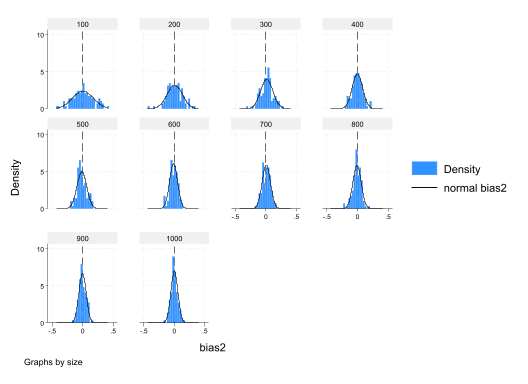
Model 2: Serial Correlation
Relax the assumption of an iid error term and allow for serial correlation. The OLS estimator is unbiased and consistent. However, the std errors are wrong since the software does not know that you have serially correlated errors and you are not taking this into account in the estimation.
\[ Y_t = \beta_1 + \beta_2X_t + \upsilon_t \qquad \text{where}\quad \upsilon_t = \rho \upsilon_{t-1}+\varepsilon_t \quad\text{and}\quad \varepsilon_t\sim N(0,\sigma^2) \] We say that \(U_t\) follows an AR(1) process. You can show that \(\hat{\beta}_2\) remains unbiased and consistant. However, the standard homoskedastic-variance estimator is incorrect:
\[ Var(\hat{\beta}_2) \neq \frac{\sigma^2}{Var(X_t)} \]
Simulation
cap prog drop mc2
program define mc2, rclass
    syntax [, obs(integer 1) s(real 1) b1(real 0) b2(real 0) bias2(real 0) sigma(real 1) rho(real 0)]
    drop _all
    set obs `obs'
    gen u=0
    gen time=_n
    tsset time
    gen e = rnormal(0,`sigma')
    forvalues i=2/`obs'  {
    replace u=`rho'*u[_n-1] + e if _n==`i'
    }
    gen x=uniform()*`s'
    gen y=`b1'+`b2'*x + u
    reg y x
    return scalar b1=_b[_cons]
    return scalar b2=_b[x]
    return scalar se2 = _se[x]
    return scalar t2 = _b[x]/_se[x]
end

simulate b1=r(b1) b2=r(b2) se2=r(se2) t2=r(t2), reps(100): mc2, obs(50) s(6) b1(4) b2(2) sigma(3) rho(0.2)
gen bias2=b2-2
su b2 t2 se2
su bias2
histogram bias2, normal xline(`r(mean)')
      Command: mc2, obs(50) s(6) b1(4) b2(2) sigma(3) rho(0.2)
           b1: r(b1)
           b2: r(b2)
          se2: r(se2)
           t2: r(t2)

Simulations (100): .........10.........20.........30.........40.........50.....
> ....60.........70.........80.........90.........100 done

    Variable |        Obs        Mean    Std. dev.       Min        Max
-------------+---------------------------------------------------------
          b2 |        100    1.975448    .2406981   1.466939   2.656462
          t2 |        100    8.010763      1.3815   4.681076   10.78957
         se2 |        100    .2500731    .0286469   .2042868   .3313515

    Variable |        Obs        Mean    Std. dev.       Min        Max
-------------+---------------------------------------------------------
       bias2 |        100   -.0245523    .2406981  -.5330607   .6564617
(bin=10, start=-.53306067, width=.11895224)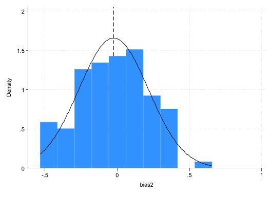
To demonstrate consistency we need to repeat the exercise for larger and larger \(n\)’s.
tempfile simdata
forvalues n = 100(100)1000 {
    simulate b1=r(b1) b2=r(b2) se2=r(se2) t2=r(t2), reps(100): mc2, obs(`n') s(6) b1(4) b2(2) sigma(3) rho(0.2)
    gen size = `n'
    if `n'==100 save `simdata', replace
    else {
        append using `simdata'
        save `simdata', replace
    }
}
gen bias2=b2-2
histogram bias2, normal xline(0) by(size)
      Command: mc2, obs(100) s(6) b1(4) b2(2) sigma(3) rho(0.2)
           b1: r(b1)
           b2: r(b2)
          se2: r(se2)
           t2: r(t2)

Simulations (100): .........10.........20.........30.........40.........50.....
> ....60.........70.........80.........90.........100 done
(file C:\Users\neil_\AppData\Local\Temp\ST_1d48_000009.tmp not found)
file C:\Users\neil_\AppData\Local\Temp\ST_1d48_000009.tmp saved as .dta
    format

      Command: mc2, obs(200) s(6) b1(4) b2(2) sigma(3) rho(0.2)
           b1: r(b1)
           b2: r(b2)
          se2: r(se2)
           t2: r(t2)

Simulations (100): .........10.........20.........30.........40.........50.....
> ....60.........70.........80.........90.........100 done
file C:\Users\neil_\AppData\Local\Temp\ST_1d48_000009.tmp saved as .dta
    format

      Command: mc2, obs(300) s(6) b1(4) b2(2) sigma(3) rho(0.2)
           b1: r(b1)
           b2: r(b2)
          se2: r(se2)
           t2: r(t2)

Simulations (100): .........10.........20.........30.........40.........50.....
> ....60.........70.........80.........90.........100 done
file C:\Users\neil_\AppData\Local\Temp\ST_1d48_000009.tmp saved as .dta
    format

      Command: mc2, obs(400) s(6) b1(4) b2(2) sigma(3) rho(0.2)
           b1: r(b1)
           b2: r(b2)
          se2: r(se2)
           t2: r(t2)

Simulations (100): .........10.........20.........30.........40.........50.....
> ....60.........70.........80.........90.........100 done
file C:\Users\neil_\AppData\Local\Temp\ST_1d48_000009.tmp saved as .dta
    format

      Command: mc2, obs(500) s(6) b1(4) b2(2) sigma(3) rho(0.2)
           b1: r(b1)
           b2: r(b2)
          se2: r(se2)
           t2: r(t2)

Simulations (100): .........10.........20.........30.........40.........50.....
> ....60.........70.........80.........90.........100 done
file C:\Users\neil_\AppData\Local\Temp\ST_1d48_000009.tmp saved as .dta
    format

      Command: mc2, obs(600) s(6) b1(4) b2(2) sigma(3) rho(0.2)
           b1: r(b1)
           b2: r(b2)
          se2: r(se2)
           t2: r(t2)

Simulations (100): .........10.........20.........30.........40.........50.....
> ....60.........70.........80.........90.........100 done
file C:\Users\neil_\AppData\Local\Temp\ST_1d48_000009.tmp saved as .dta
    format

      Command: mc2, obs(700) s(6) b1(4) b2(2) sigma(3) rho(0.2)
           b1: r(b1)
           b2: r(b2)
          se2: r(se2)
           t2: r(t2)

Simulations (100): .........10.........20.........30.........40.........50.....
> ....60.........70.........80.........90.........100 done
file C:\Users\neil_\AppData\Local\Temp\ST_1d48_000009.tmp saved as .dta
    format

      Command: mc2, obs(800) s(6) b1(4) b2(2) sigma(3) rho(0.2)
           b1: r(b1)
           b2: r(b2)
          se2: r(se2)
           t2: r(t2)

Simulations (100): .........10.........20.........30.........40.........50.....
> ....60.........70.........80.........90.........100 done
file C:\Users\neil_\AppData\Local\Temp\ST_1d48_000009.tmp saved as .dta
    format

      Command: mc2, obs(900) s(6) b1(4) b2(2) sigma(3) rho(0.2)
           b1: r(b1)
           b2: r(b2)
          se2: r(se2)
           t2: r(t2)

Simulations (100): .........10.........20.........30.........40.........50.....
> ....60.........70.........80.........90.........100 done
file C:\Users\neil_\AppData\Local\Temp\ST_1d48_000009.tmp saved as .dta
    format

      Command: mc2, obs(1000) s(6) b1(4) b2(2) sigma(3) rho(0.2)
           b1: r(b1)
           b2: r(b2)
          se2: r(se2)
           t2: r(t2)

Simulations (100): .........10.........20.........30.........40.........50.....
> ....60.........70.........80.........90.........100 done
file C:\Users\neil_\AppData\Local\Temp\ST_1d48_000009.tmp saved as .dta
    format
Model 3: Dynamic model without serial correlation
Consider a version of Model 1, where the regressor is the lag of the dependent variable. \[ Y_t = \beta_1 + \beta_2Y_{t-1} + \upsilon_t \qquad \text{with}\quad \upsilon_t\sim N(0,\sigma^2) \] The OLS estimator is now, \[ \hat{\beta}_2 = \beta_2 + \frac{\sum_t \tilde{Y}_{t-1}\tilde{\upsilon}_t}{\sum_t \tilde{Y}_{t-1}^2} \] This model is biased, since
\[ E\bigg[\frac{\sum_t \tilde{Y}_{t-1}\tilde{\upsilon}_t}{\sum_t \tilde{Y}_{t-1}^2}\bigg] \neq \frac{E\big[\sum_t \tilde{Y}_{t-1}\tilde{\upsilon}_t\big]}{E\big[\sum_t \tilde{Y}_{t-1}^2\big]} \] When the regressor was \(X_t\), the above statement was true given the Law of Iterated Expectations. However, you can use Slutsky’s theorem and the WLLN to show that \(\hat{\beta}_2\rightarrow_p \beta_2\). This result relies on the fact that \(Y_{t-1}\) is realized before \(\upsilon_t\) which is iid. Thus, the bias goes to 0 as \(n\rightarrow \infty\).
Simulation
cap prog drop mc3
program define mc3, rclass
    syntax [, obs(integer 1)  b1(real 0)  b2(real 0)  sigma(real 1)]
    drop _all
    set obs `obs'
    gen y=0
    gen u = rnormal(0,`sigma')
    gen time=_n
    tsset time
    forvalues i=2/`obs'  {
    replace y=`b1'+ `b2'* y[_n-1] + u  if _n==`i'
    }
    reg y  L.y
    return scalar b1=_b[_cons]
    return scalar b2=_b[L.y]
    return scalar se2 = _se[L.y]
  return scalar t2 = _b[L.y]/_se[L.y]
end


simulate b1=r(b1) b2=r(b2) se2=r(se2) t2=r(t2), reps(100): mc3, obs(50) b1(4)  b2(0.2) sigma(3)
gen bias2=b2-0.2
sum b2 t2 se2
sum bias2
histogram bias2, normal xline(`r(mean)')
      Command: mc3, obs(50) b1(4) b2(0.2) sigma(3)
           b1: r(b1)
           b2: r(b2)
          se2: r(se2)
           t2: r(t2)

Simulations (100): .........10.........20.........30.........40.........50.....
> ....60.........70.........80.........90.........100 done

    Variable |        Obs        Mean    Std. dev.       Min        Max
-------------+---------------------------------------------------------
          b2 |        100     .167145    .1275283  -.1321701   .4612297
          t2 |        100    1.213486    .9468185  -.9446563   3.532131
         se2 |        100    .1400517    .0042463   .1278178   .1539907

    Variable |        Obs        Mean    Std. dev.       Min        Max
-------------+---------------------------------------------------------
       bias2 |        100    -.032855    .1275283  -.3321701   .2612297
(bin=10, start=-.33217007, width=.05933998)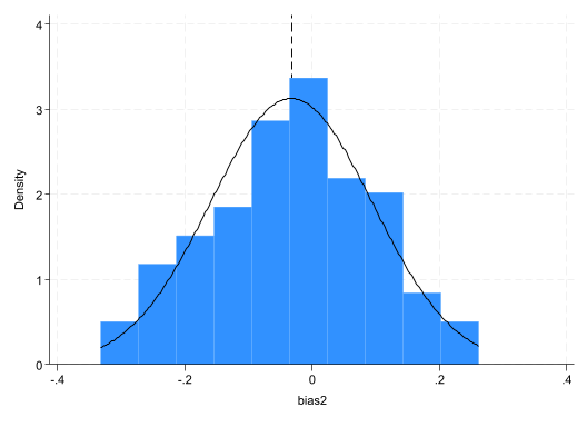
To demonstrate consistency we need to repeat the exercise for larger and larger \(n\)’s.
tempfile simdata
forvalues n = 100(100)1000 {
    simulate b1=r(b1) b2=r(b2) se2=r(se2) t2=r(t2), reps(100): mc3, obs(`n') b1(4) b2(0.2) sigma(3)
    gen size = `n'
    if `n'==100 save `simdata', replace
    else {
        append using `simdata'
        save `simdata', replace
    }
}
gen bias2=b2-0.2
histogram bias2, normal xline(0) by(size)
      Command: mc3, obs(100) b1(4) b2(0.2) sigma(3)
           b1: r(b1)
           b2: r(b2)
          se2: r(se2)
           t2: r(t2)

Simulations (100): .........10.........20.........30.........40.........50.....
> ....60.........70.........80.........90.........100 done
(file C:\Users\neil_\AppData\Local\Temp\ST_1d48_00000d.tmp not found)
file C:\Users\neil_\AppData\Local\Temp\ST_1d48_00000d.tmp saved as .dta
    format

      Command: mc3, obs(200) b1(4) b2(0.2) sigma(3)
           b1: r(b1)
           b2: r(b2)
          se2: r(se2)
           t2: r(t2)

Simulations (100): .........10.........20.........30.........40.........50.....
> ....60.........70.........80.........90.........100 done
file C:\Users\neil_\AppData\Local\Temp\ST_1d48_00000d.tmp saved as .dta
    format

      Command: mc3, obs(300) b1(4) b2(0.2) sigma(3)
           b1: r(b1)
           b2: r(b2)
          se2: r(se2)
           t2: r(t2)

Simulations (100): .........10.........20.........30.........40.........50.....
> ....60.........70.........80.........90.........100 done
file C:\Users\neil_\AppData\Local\Temp\ST_1d48_00000d.tmp saved as .dta
    format

      Command: mc3, obs(400) b1(4) b2(0.2) sigma(3)
           b1: r(b1)
           b2: r(b2)
          se2: r(se2)
           t2: r(t2)

Simulations (100): .........10.........20.........30.........40.........50.....
> ....60.........70.........80.........90.........100 done
file C:\Users\neil_\AppData\Local\Temp\ST_1d48_00000d.tmp saved as .dta
    format

      Command: mc3, obs(500) b1(4) b2(0.2) sigma(3)
           b1: r(b1)
           b2: r(b2)
          se2: r(se2)
           t2: r(t2)

Simulations (100): .........10.........20.........30.........40.........50.....
> ....60.........70.........80.........90.........100 done
file C:\Users\neil_\AppData\Local\Temp\ST_1d48_00000d.tmp saved as .dta
    format

      Command: mc3, obs(600) b1(4) b2(0.2) sigma(3)
           b1: r(b1)
           b2: r(b2)
          se2: r(se2)
           t2: r(t2)

Simulations (100): .........10.........20.........30.........40.........50.....
> ....60.........70.........80.........90.........100 done
file C:\Users\neil_\AppData\Local\Temp\ST_1d48_00000d.tmp saved as .dta
    format

      Command: mc3, obs(700) b1(4) b2(0.2) sigma(3)
           b1: r(b1)
           b2: r(b2)
          se2: r(se2)
           t2: r(t2)

Simulations (100): .........10.........20.........30.........40.........50.....
> ....60.........70.........80.........90.........100 done
file C:\Users\neil_\AppData\Local\Temp\ST_1d48_00000d.tmp saved as .dta
    format

      Command: mc3, obs(800) b1(4) b2(0.2) sigma(3)
           b1: r(b1)
           b2: r(b2)
          se2: r(se2)
           t2: r(t2)

Simulations (100): .........10.........20.........30.........40.........50.....
> ....60.........70.........80.........90.........100 done
file C:\Users\neil_\AppData\Local\Temp\ST_1d48_00000d.tmp saved as .dta
    format

      Command: mc3, obs(900) b1(4) b2(0.2) sigma(3)
           b1: r(b1)
           b2: r(b2)
          se2: r(se2)
           t2: r(t2)

Simulations (100): .........10.........20.........30.........40.........50.....
> ....60.........70.........80.........90.........100 done
file C:\Users\neil_\AppData\Local\Temp\ST_1d48_00000d.tmp saved as .dta
    format

      Command: mc3, obs(1000) b1(4) b2(0.2) sigma(3)
           b1: r(b1)
           b2: r(b2)
          se2: r(se2)
           t2: r(t2)

Simulations (100): .........10.........20.........30.........40.........50.....
> ....60.........70.........80.........90.........100 done
file C:\Users\neil_\AppData\Local\Temp\ST_1d48_00000d.tmp saved as .dta
    format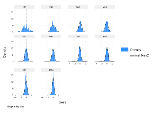
Model 4: Dynamic model with serial correlation
Consider a version of Model 2, where the regressor is the lag of the dependent variable. \[ Y_t = \beta_1 + \beta_2Y_{t-1} + \upsilon_t \text{where}\quad \upsilon_t = \rho \upsilon_{t-1}+\varepsilon_t \quad\text{and}\quad \varepsilon_t\sim N(0,\sigma^2) \] As with model 3, the OLS estimator will be biased. In addition, since \(Cov(\upsilon_t,\upsilon_{t-1})\neq0\) and \(Cov(Y_t,\upsilon_{t})\neq 0\) (for any \(t\)), \[ \Rightarrow Cov(Y_{t-1},\upsilon_{t})\neq 0 \] As a result \(\hat{\beta}_2\) is inconsistent.
Simulation
cap prog drop mc4
program define mc4, rclass
    syntax [, obs(integer 1)  b1(real 0)  b2(real 0)  sigma(real 1) rho(real 0) ]
    drop _all
    set obs `obs'
    gen y=0
    gen u=0
    gen e = rnormal(0,`sigma')
    gen time=_n
    tsset time

    forvalues i=2/`obs'  {
    replace u=`rho'*u[_n-1] + e if _n==`i'
    replace y=`b1'+ `b2'* y[_n-1] + u  if _n==`i'
    }
    reg y  L.y
    return scalar b1=_b[_cons]
    return scalar b2=_b[L.y]
    return scalar se2 = _se[L.y]
  return scalar t2 = _b[L.y]/_se[L.y]
end

simulate b1=r(b1) b2=r(b2) se2=r(se2) t2=r(t2), reps(100): mc4, obs(50) b1(4) b2(0.2) sigma(3) rho(0.2)
gen bias2=b2-0.2
sum b2 t2 se2
sum bias2
histogram bias2, normal xline(`r(mean)')
      Command: mc4, obs(50) b1(4) b2(0.2) sigma(3) rho(0.2)
           b1: r(b1)
           b2: r(b2)
          se2: r(se2)
           t2: r(t2)

Simulations (100): .........10.........20.........30.........40.........50.....
> ....60.........70.........80.........90.........100 done

    Variable |        Obs        Mean    Std. dev.       Min        Max
-------------+---------------------------------------------------------
          b2 |        100    .3424452    .1554043  -.1707231   .6607195
          t2 |        100    2.666883    1.363437  -1.216084   6.210446
         se2 |        100    .1323436    .0083629   .1063884   .1438691

    Variable |        Obs        Mean    Std. dev.       Min        Max
-------------+---------------------------------------------------------
       bias2 |        100    .1424452    .1554043  -.3707231   .4607195
(bin=10, start=-.37072313, width=.08314427)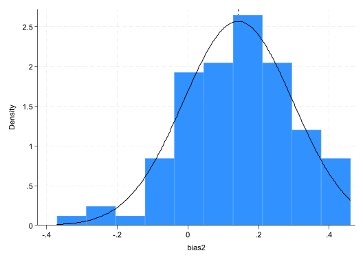
To demonstrate consistency we need to repeat the exercise for larger and larger \(n\)’s.
tempfile simdata
forvalues n = 100(100)1000 {
    simulate b1=r(b1) b2=r(b2) se2=r(se2) t2=r(t2), reps(100): mc4, obs(`n') b1(4) b2(0.2) sigma(3) rho(0.2)
    gen size = `n'
    if `n'==100 save `simdata', replace
    else {
        append using `simdata'
        save `simdata', replace
    }
}
gen bias2=b2-0.2
histogram bias2, normal xline(0) by(size)
      Command: mc4, obs(100) b1(4) b2(0.2) sigma(3) rho(0.2)
           b1: r(b1)
           b2: r(b2)
          se2: r(se2)
           t2: r(t2)

Simulations (100): .........10.........20.........30.........40.........50.....
> ....60.........70.........80.........90.........100 done
(file C:\Users\neil_\AppData\Local\Temp\ST_1d48_00000h.tmp not found)
file C:\Users\neil_\AppData\Local\Temp\ST_1d48_00000h.tmp saved as .dta
    format

      Command: mc4, obs(200) b1(4) b2(0.2) sigma(3) rho(0.2)
           b1: r(b1)
           b2: r(b2)
          se2: r(se2)
           t2: r(t2)

Simulations (100): .........10.........20.........30.........40.........50.....
> ....60.........70.........80.........90.........100 done
file C:\Users\neil_\AppData\Local\Temp\ST_1d48_00000h.tmp saved as .dta
    format

      Command: mc4, obs(300) b1(4) b2(0.2) sigma(3) rho(0.2)
           b1: r(b1)
           b2: r(b2)
          se2: r(se2)
           t2: r(t2)

Simulations (100): .........10.........20.........30.........40.........50.....
> ....60.........70.........80.........90.........100 done
file C:\Users\neil_\AppData\Local\Temp\ST_1d48_00000h.tmp saved as .dta
    format

      Command: mc4, obs(400) b1(4) b2(0.2) sigma(3) rho(0.2)
           b1: r(b1)
           b2: r(b2)
          se2: r(se2)
           t2: r(t2)

Simulations (100): .........10.........20.........30.........40.........50.....
> ....60.........70.........80.........90.........100 done
file C:\Users\neil_\AppData\Local\Temp\ST_1d48_00000h.tmp saved as .dta
    format

      Command: mc4, obs(500) b1(4) b2(0.2) sigma(3) rho(0.2)
           b1: r(b1)
           b2: r(b2)
          se2: r(se2)
           t2: r(t2)

Simulations (100): .........10.........20.........30.........40.........50.....
> ....60.........70.........80.........90.........100 done
file C:\Users\neil_\AppData\Local\Temp\ST_1d48_00000h.tmp saved as .dta
    format

      Command: mc4, obs(600) b1(4) b2(0.2) sigma(3) rho(0.2)
           b1: r(b1)
           b2: r(b2)
          se2: r(se2)
           t2: r(t2)

Simulations (100): .........10.........20.........30.........40.........50.....
> ....60.........70.........80.........90.........100 done
file C:\Users\neil_\AppData\Local\Temp\ST_1d48_00000h.tmp saved as .dta
    format

      Command: mc4, obs(700) b1(4) b2(0.2) sigma(3) rho(0.2)
           b1: r(b1)
           b2: r(b2)
          se2: r(se2)
           t2: r(t2)

Simulations (100): .........10.........20.........30.........40.........50.....
> ....60.........70.........80.........90.........100 done
file C:\Users\neil_\AppData\Local\Temp\ST_1d48_00000h.tmp saved as .dta
    format

      Command: mc4, obs(800) b1(4) b2(0.2) sigma(3) rho(0.2)
           b1: r(b1)
           b2: r(b2)
          se2: r(se2)
           t2: r(t2)

Simulations (100): .........10.........20.........30.........40.........50.....
> ....60.........70.........80.........90.........100 done
file C:\Users\neil_\AppData\Local\Temp\ST_1d48_00000h.tmp saved as .dta
    format

      Command: mc4, obs(900) b1(4) b2(0.2) sigma(3) rho(0.2)
           b1: r(b1)
           b2: r(b2)
          se2: r(se2)
           t2: r(t2)

Simulations (100): .........10.........20.........30.........40.........50.....
> ....60.........70.........80.........90.........100 done
file C:\Users\neil_\AppData\Local\Temp\ST_1d48_00000h.tmp saved as .dta
    format

      Command: mc4, obs(1000) b1(4) b2(0.2) sigma(3) rho(0.2)
           b1: r(b1)
           b2: r(b2)
          se2: r(se2)
           t2: r(t2)

Simulations (100): .........10.........20.........30.........40.........50.....
> ....60.........70.........80.........90.........100 done
file C:\Users\neil_\AppData\Local\Temp\ST_1d48_00000h.tmp saved as .dta
    format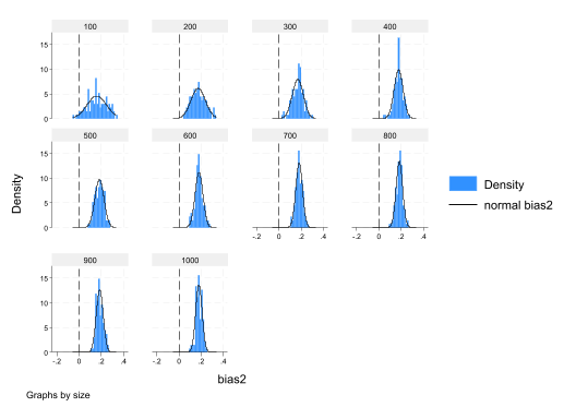
Postamble
log close